The key question to be answered by the high-level control system for a stepper motor is, when should the next step be taken? While this almost always depends on the application, the similarities between different applications are sufficient to justify the development of fairly complex general purpose stepper motor controllers.
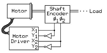
Stepper motor control may be based on open loop or closed loop models. We are primarily interested in open loop models, because this is where stepper motors excel, but we will treat closed loop models briefly because they are somewhat simpler. Figure 1 illustrates an extreme example:

In Figure 1, a quadrature shaft encoder is attached to the drive shaft of a permanent magnet or hybrid stepper motor, and the two phase output of this encoder is used to directly generate the control vector for the motor driver.
Rotary shaft encoders are typically rated in output pulses per channel per revolution; for this example to be useful, for a motor with n steps per revolution, the shaft encoder output must give n / 2 pulses per channel per revolution. If this is the case, the behavior of this system will depend on how the shaft encoder is rotated around the motor shaft relative to the motor.
If the shaft encoder is rotated into a position where the output of the shaft encoder translates to a control vector that holds the motor shaft in its initial position, the motor shaft will not rotate of itself, and if the motor shaft is rotated by force, it will stay wherever it is left. We will refer to this position of the shaft encoder relative to the motor as the neutral position.
If the shaft encoder is rotated one step clockwise (or counterclockwise) from the neutral position, the control vector output by the shaft encoder will pull the rotor clockwise (or counterclockwise). As the rotor turns, the shaft encoder will change the control vector so that the rotor is always trying to maintain a position one step clockwise (or counterclockwise) from where it is at the moment. The torque produced by this method will fall off with rotor speed, but this control system will always produce the maximum torque the motor is able to deliver at any speed.
In effect, with this one-step displacement, we have constructed a brushless DC motor from a stepper motor and a collection of off-the-shelf parts. In practice, this is rarely done, but there are numerous applications of stepper motors in closed-loop control systems that are based on this model, usually with a microprocessor included in the feedback loop between the shaft encoder and the motor controller.
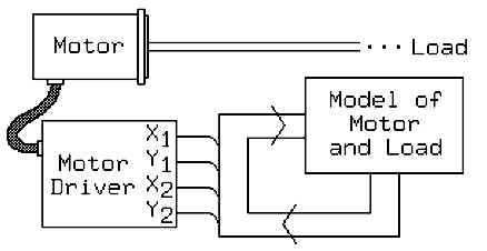
In an open-loop control system, this feedback loop is broken, but at a high level, the basic principle remains quite similar, as illustrated in Figure 2:

In Figure 2, we replace the shaft encoder from Figure 1 with a simulation model of the response of the motor and load to the control vector. At any instant, the actual position of the rotor is unknown! Nonetheless, we can use the simulation model to predict, based on an assumed rotor position and velocity, how the motor will respond to the control vector, and we can construct this model so that its output is the control vector generated by a simulated shaft encoder.
So long as the model is sufficiently accurate, the behavior of the motor controlled by this model will be the same as the behavior of the motor controlled by a closed loop system!
Model Variables
In the example given in Figure 1, the only control variable offered is the angle of the shaft encoder relative to the motor. In effect, this controls the extent to which the equilibrium point of the motor’s torque versus shaft angle curve leads or follows the current rotor position. In theory, any desired motor behavior can be elicited by adjusting this angle, but it is far more convenient to speak in terms of other variables:
Θ – The predicted shaft position (radians)
Θtarget – The target shaft position determined by the application
V = dΘ / dt – The predicted velocity (radians per second)
Vtarget – The target velocity determined by the application
A = dV / dt – The predicted acceleration (radians per second squared)
Atarget – The target acceleration, may be determined by the application
The basic motor characteristics:
S – step or microstep angle, in radians
μ – moment of inertia of rotor and load
h – the holding torque of the motor
Note that here, the step angle S is not the physical step angle of the motor, but rather, the step angle offered by the mid-level motor interface; this may be a full step, a half step, or a microstep of some size!
Models
The simplest model that will do the job is almost always the best. For some applications, this means the model is so simple that it is hard to identify it as a model! For example, consider the case where the application demands a constant motor velocity:
Atarget = 0
Vtarget = Constant in this case, tstep = S / Vtarget
Where
tstep – time per step
This barely looks like a model; in part, this is because we have omitted the statement that, every tstep seconds, we advance the control vector one step:
repeat the following cycle forever:
wait tstep seconds and then
Θ = Θ + S
step ( 1 )
A more interesting model is required if we want to maintain a constant acceleration. Obviously, we can’t do this forever, but we’ll use this model as a component in more complex models that require changes of velocity or position. In this case, Atarget = Constant
Where
Atarget < h / μ
In developing a model, we begin with the observation that, for constant acceleration A and assuming a standing start at time 0, Θ = 1/2 A t2
More generally, if the motor starts at position Θ and velocity V, after time t the new position Θ’ and velocity V’ will be: Θ’ = 1/2 A t2 + V t Θ V’ = A t + V
Setting Θ = 0 and Θ’ = S, we solve first for t, the time taken to move one step, as a function of V and A:
1/2 A t2 + V t – S = 0
t = (-V ± (V2 + 2 A S)0.5) / A
Here, we have applied the quadratic formula, and for our situation, this gives two real roots! The additive root is the root we are concerned with; for this, we can use the resulting time to compute the velocity at the end of one step: tstep = (-V + (V2 + 2 A S)0.5) / A
V’ = (V2 + 2 A S )0.5
We can combine this model for acceleration with the model for constant speed running to make a motor controller that will seek Vtarget, assuming that an outside agent may change Vtarget at any time:
repeat the following cycle forever:
if V = Vtarget do the following:
wait S / Vtarget seconds and then
Θ = Θ + S
step( 1 )
otherwise, if V < Vtarget, accelerate as follows:
wait (-V + (V2 + 2 Aaccel S)0.5 ) / Aaccel seconds and then
Θ = Θ + S
V = (V2 + 2 Aaccel S)0.5
step ( 1 )
otherwise, V > Vtarget, decelerate as follows:
wait ( -V + (V2 + 2 Adecel S)0.5 ) / Adecel seconds and then
Θ =Θ + S
V = (V2 + 2 Adecel S)0.5
step ( 1 )
This control system is not fully satisfactory for a number of reasons! First, it only allows the motor to operate in one direction and it fails utterly when V reaches zero; at that point, if a divide by zero operation is allowed to produce an infinite result, the program will wait infinitely and never again respond to change in the control input.
The second shortcoming of this program is simpler to correct: As written, there is an infinitesimal probability of the motor speed reaching the desired speed and staying there with Vtarget equal to V. Far more likely, what will happen is that V will oscillate around Vtarget, taking alternate accelerating and decelerating steps and never settling down at the desired running speed.
A quick and dirty solution to this latter problem is to add code to recognize when V passes Vtarget during acceleration or deceleration; when this occurs, V can be set to Vtarget. Formally, this is incorrect, but if the acceleration and deceleration rates are not too high and if there is sufficient damping in the system, this will work quite well.
In a frictionless system using sine-cosine microstepping at speeds below the cut of speed for the motor, the available torque is effectively constant and we can use the full torque to accelerate 0r decelerate the motor, so the above control algorithm will work with Aaccel = Adecel = h / μ.
If there is significant static friction, we can take this into account as follows: Aaccel= (h – f) / μ
Adecel = (h + f) / μ
Where
F – frictional torque If the motor is run using the maximum available acceleration and declaration, any unexpected increase in the load will cause the motor rotor to fall behind its predicted position, and the result will be a failure of the control system. As a result, open-loop stepper motor control systems are never run at the accelerations give above! In the case of fill or half-stepping, where there is no sine-cosine torque compensation, the available torque varies over a range of a factor of 20.5, so we typically adjust the accelerations given above by this amount: Ace=((h / 1.414) – f) / μ
Adecel = ((h / 1.414) + f) / μ
If we operate consistently near the edge of the performance envelope, and if we never request a velocity Vtarget near the resonant speed of the motor, we can safely accelerate through resonances without relying on damping. If, on the other hand, we select acceleration values that are significantly below the maximum that is possible, electrical or mechanical damping may be needed to avoid problems with resonance.
Note that it is not difficult to extend the above control model to account, at least approximately, for viscous fiction and for the drop off of torque as a function of speed. To do this, we merely modify the above formulas for Aaccel and Adecel so that h and f are functions of V. Thus, instead of treating these as constants of the control algorithm, we must recomputed the available acceleration at each step.
If our goal is to turn the motor smoothly from one set position to another, we must first accelerate it, then perhaps coast at fixed speed for a while, then decelerate. The decision governing when to begin decelerating rests on a knowledge of the stopping distance from any particular velocity. Assuming that the available acceleration is constant over the relevant range of speeds, we can compute this from: V= Adecel t
Θ = 1/2 Adecel t2
First we solve for the stopping time, t= V / Adecel and then we solve for the stopping angle Θ = 1/2 Adecel ( V / Adecel)2 = V2 / ( 2 Adecel)
Given this, we can outline a procedure for moving the motor from its current estimated position to a step just beyond some target position:
moveto (Θtarget )
– a function of one argument O
– no value is returned
while V < Vtarget
and while Θ < Θtarget – V2 / (2 Adecel) repeat the following to accelerate
step ( 1 )
wait (-V + (V2 + 2 Aaccel S)0.5) / Aaccel seconds and then
Θ =Θ + S
V = (V2+ 2 Aaccel S)0.5
V = Vtarget
While Θ <Θtarget – V2 / ( 2 Adecel ) repeat the following to coast
step ( 1 )
wait S / Vtarget seconds and then
Θ = Θ + S
while Θ < Θtarget repeat the following to decelerate
step ( 1 )
wait ( -V + ( V2 + 2 Adecel S )0.5 ) / Aaccel seconds and then
Θ = Θ + S
V = (V2 + 2 Aaccel S )0.5
V = 0
done, Θ and Θtarget are within a step of each other!
The control model only moves the motor one direction, it fails to plan in terms of the quantization of available stopping positions, and it doesn’t account for the cyclic nature of Θ. Nonetheless, it is a useful illustration. Note that we have used V target as a limiting velocity in this code, but that this will only be relevant during long moves; for short moves, the motor will never reach this speed.
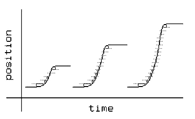
With the above, code, so long as the acceleration and deceleration rates are high enough to avoid dwelling for too long at resonant speeds, and so long as Vtarget is not too close to a resonant speed, a plot of rotor position versus time will show fairly clean moves, as illustrated in Figure 3:

If the motor is to be accelerated at the maximum possible rate, the control model used above is not sufficient. In that case, during acceleration, the equilibrium position must be maintained between 0.5 and 1.5 steps ahead of the rotor position as the rotor moves, and during deceleration, the equilibrium position must be maintained the same distance behind the rotor position. This requires careful logic at the turnaround point, when the change is made from accelerating to decelerating modes. The above control model omits any such considerations, but it is adequate at accelerations sufficiently below the maximum available!